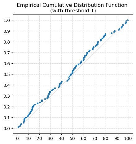
`eda_stats_utils`

Utility Functions that can be used for exploratory data analysis and statistics. Includes all stable utility functions for eda and statistics.

Data analysis plots

source

ecdf

 ecdf (data:pandas.core.series.Series|numpy.ndarray,
       threshold:Optional[int]=None,
       figsize:Optional[tuple[int,int]]=None)

Compute Empirical Cumulative Distribution Function (ECDF), plot it and returns values.

	Type	Default	Details
data	pd.Series \| np.ndarray		data to analyse
threshold	Optional[int]	None	cummulative frequency used as threshold. Must be between 0 and 1
figsize	Optional[tuple[int, int]]	None	figure size (width, height)
Returns	tuple[np.array, np.array, int]		sorted data (ascending), cumulative frequencies, last index

ecdf plots the empirical cumulative distribution function (ECDF), for data cumulative frequencies from 0 to threshold <= 1.

The empirical cumulative distribution function (ECDF) is a step function that jumps up by 1/n at each of the n data points in the dataset. Its value at any specified value of the measured variable is the fraction of observations of the measured variable that are less than or equal to the specified value.

The ECDF is an estimate of the cumulative distribution function that generated the points in the sample. It allows to compare with the distribution that is expected.

df = pd.DataFrame(data={'a': np.random.random(100) * 100,'b': np.random.random(100) * 50,'c': np.random.random(100)})
data_1, freq_1, last_idx_1 = ecdf(data=df.a, threshold=1, figsize=(5, 5))

data_2, freq_2, last_idx_2 = ecdf(data=df.a, threshold=0.75, figsize=(5, 5))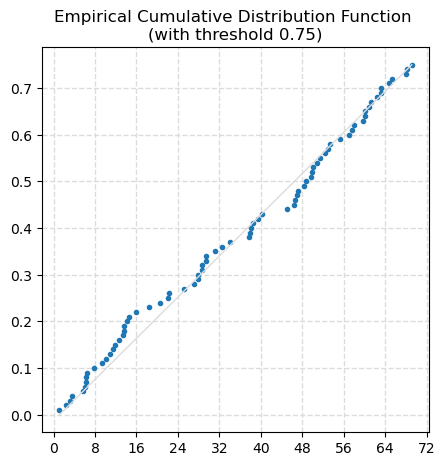

data_3, freq_3, last_idx_3 = ecdf(data=df.a, threshold=0.5, figsize=(5, 5))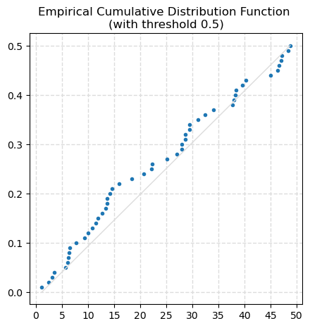

The ecdf function also returns: - the data used for the ECDF, with values sorted from smallest to largest - the respective cummulative frequencies - the index of data value/frequency plotted (at the threshold)

data_1

array([ 0.85,  2.1 ,  2.44,  3.22,  3.24,  3.9 ,  4.65,  5.53,  6.08,  6.34,  6.84,  6.98,  8.37,  9.09, 12.58, 12.96,
       13.62, 14.5 , 15.06, 17.11, 17.52, 17.99, 19.12, 22.3 , 22.45, 23.87, 23.87, 24.15, 24.28, 25.95, 26.79, 30.31,
       30.4 , 34.83, 38.01, 38.56, 38.62, 39.47, 39.58, 41.1 , 42.43, 43.57, 43.73, 45.92, 47.19, 47.66, 48.52, 49.03,
       49.6 , 49.98, 51.07, 52.14, 53.06, 53.92, 54.66, 55.88, 56.12, 56.29, 56.52, 57.02, 57.63, 58.54, 59.37, 62.65,
       62.91, 62.93, 63.22, 64.12, 64.82, 65.06, 65.35, 67.16, 70.6 , 70.94, 72.24, 72.45, 73.87, 74.91, 78.44, 79.17,
       79.78, 79.82, 82.53, 84.96, 85.14, 85.43, 86.19, 86.35, 88.31, 89.76, 90.42, 91.69, 93.11, 96.71, 97.38, 98.32,
       98.33, 98.37, 98.56, 98.83])

freq_1

array([0.01, 0.02, 0.03, 0.04, 0.05, 0.06, 0.07, 0.08, 0.09, 0.1 , 0.11, 0.12, 0.13, 0.14, 0.15, 0.16, 0.17, 0.18,
       0.19, 0.2 , 0.21, 0.22, 0.23, 0.24, 0.25, 0.26, 0.27, 0.28, 0.29, 0.3 , 0.31, 0.32, 0.33, 0.34, 0.35, 0.36,
       0.37, 0.38, 0.39, 0.4 , 0.41, 0.42, 0.43, 0.44, 0.45, 0.46, 0.47, 0.48, 0.49, 0.5 , 0.51, 0.52, 0.53, 0.54,
       0.55, 0.56, 0.57, 0.58, 0.59, 0.6 , 0.61, 0.62, 0.63, 0.64, 0.65, 0.66, 0.67, 0.68, 0.69, 0.7 , 0.71, 0.72,
       0.73, 0.74, 0.75, 0.76, 0.77, 0.78, 0.79, 0.8 , 0.81, 0.82, 0.83, 0.84, 0.85, 0.86, 0.87, 0.88, 0.89, 0.9 ,
       0.91, 0.92, 0.93, 0.94, 0.95, 0.96, 0.97, 0.98, 0.99, 1.  ])

The function returns all the sorted data and frequencies, independently from the threshold. In the example above, data_1 and data_2 have the same values.

np.array_equal(data_1, data_2), np.array_equal(freq_1, freq_2)

(True, True)

data_2[:last_idx_2+1]

array([ 0.85,  2.1 ,  2.44,  3.22,  3.24,  3.9 ,  4.65,  5.53,  6.08,  6.34,  6.84,  6.98,  8.37,  9.09, 12.58, 12.96,
       13.62, 14.5 , 15.06, 17.11, 17.52, 17.99, 19.12, 22.3 , 22.45, 23.87, 23.87, 24.15, 24.28, 25.95, 26.79, 30.31,
       30.4 , 34.83, 38.01, 38.56, 38.62, 39.47, 39.58, 41.1 , 42.43, 43.57, 43.73, 45.92, 47.19, 47.66, 48.52, 49.03,
       49.6 , 49.98, 51.07, 52.14, 53.06, 53.92, 54.66, 55.88, 56.12, 56.29, 56.52, 57.02, 57.63, 58.54, 59.37, 62.65,
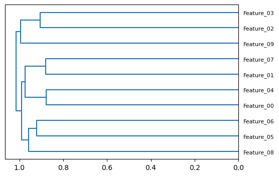
       62.91, 62.93, 63.22, 64.12, 64.82, 65.06, 65.35, 67.16, 70.6 , 70.94, 72.24])

source

cluster_columns

Plot dendogram based on Dataframe’s columns’ spearman correlation coefficients

This function was first seen on fastai repo

feats = [f"Feature_{i:02d}" for i in range(10)]
print('Features:')
print(', '.join(feats))
X = pd.DataFrame(np.random.normal(size=(500, 10)), columns=feats)
cluster_columns(X, (6, 4), 8)

Features:
Feature_00, Feature_01, Feature_02, Feature_03, Feature_04, Feature_05, Feature_06, Feature_07, Feature_08, Feature_09